Justice and Bargaining
J. McKenzie Alexander and B. Skyrms, Bargaining with Neighbors: Is Justice Contagious, Journal of Philosophy 96 (11):588 (1999)
See also J. Alexander, Evolutionary Game Theory, Stanford Encyclopedia of Philosophy
Bargaining
Two individuals are to decide how to distribute a certain amount of money.
Neither is especially entitled, or especially needy, or especially anything—their positions are entirely symmetric.
Their utilities derived from the distribution may be taken, for all intents and purposes, simply as the amount of money received.
If they cannot decide, the money remains undistributed and neither gets any.
Two Principles of Justice
Optimality: a distribution is not just if, under an alternative distribution, all recipients would be better off.
Equity: if the position of the recipients is symmetric, then the distribution should be symmetric. That is to say, it does not vary when we switch the recipients.
Classical Game Theory
Suppose that two rational agents play the divide-the-dollar game. Their rationality is common knowledge. What do they do?
|
\(0\) |
\(1\) |
\(2\) |
\(3\) |
\(4\) |
\(5\) |
\(6\) |
\(7\) |
\(8\) |
\(9\) |
\(10\) |
|---|---|---|---|---|---|---|---|---|---|---|---|
\(0\) |
\(0,0\) |
\(0,1\) |
\(0,2\) |
\(0,3\) |
\(0,4\) |
\(0,5\) |
\(0,6\) |
\(0,7\) |
\(0,8\) |
\(0,9\) |
\(0,10\) |
\(1\) |
\(1,0\) |
\(1,1\) |
\(1,2\) |
\(1,3\) |
\(1,4\) |
\(1,5\) |
\(1,6\) |
\(1,7\) |
\(1,8\) |
\(1,9\) |
\(0,0\) |
\(2\) |
\(2,0\) |
\(2,1\) |
\(2,2\) |
\(2,3\) |
\(2,4\) |
\(2,5\) |
\(2,6\) |
\(2,7\) |
\(2,8\) |
\(0,0\) |
\(0,0\) |
\(3\) |
\(3,0\) |
\(3,1\) |
\(3,2\) |
\(3,3\) |
\(3,4\) |
\(3,5\) |
\(3,6\) |
\(3,7\) |
\(0,0\) |
\(0,0\) |
\(0,0\) |
\(4\) |
\(4,0\) |
\(4,1\) |
\(4,2\) |
\(4,3\) |
\(4,4\) |
\(4,5\) |
\(4,6\) |
\(0,0\) |
\(0,0\) |
\(0,0\) |
\(0,0\) |
\(5\) |
\(5,0\) |
\(5,1\) |
\(5,2\) |
\(5,3\) |
\(5,4\) |
\(5,5\) |
\(0,0\) |
\(0,0\) |
\(0,0\) |
\(0,0\) |
\(0,0\) |
\(6\) |
\(6,0\) |
\(6,1\) |
\(6,2\) |
\(6,3\) |
\(6,4\) |
\(0,0\) |
\(0,0\) |
\(0,0\) |
\(0,0\) |
\(0,0\) |
\(0,0\) |
\(7\) |
\(7,0\) |
\(7,1\) |
\(7,2\) |
\(7,3\) |
\(0,0\) |
\(0,0\) |
\(0,0\) |
\(0,0\) |
\(0,0\) |
\(0,0\) |
\(0,0\) |
\(8\) |
\(8,0\) |
\(8,1\) |
\(8,2\) |
\(0,0\) |
\(0,0\) |
\(0,0\) |
\(0,0\) |
\(0,0\) |
\(0,0\) |
\(0,0\) |
\(0,0\) |
\(9\) |
\(9,0\) |
\(9,1\) |
\(0,0\) |
\(0,0\) |
\(0,0\) |
\(0,0\) |
\(0,0\) |
\(0,0\) |
\(0,0\) |
\(0,0\) |
\(0,0\) |
\(10\) |
\(10,0\) |
\(0,0\) |
\(0,0\) |
\(0,0\) |
\(0,0\) |
\(0,0\) |
\(0,0\) |
\(0,0\) |
\(0,0\) |
\(0,0\) |
\(0,0\) |
import nashpy as nash
import numpy as np

A = np.array([[0, 0, 0, 0, 0, 0, 0, 0, 0, 0, 0],
              [1, 1, 1, 1, 1, 1, 1, 1, 1, 1, 0],
              [2, 2, 2, 2, 2, 2, 2, 2, 2, 0, 0],
              [3, 3, 3, 3, 3, 3, 3, 3, 0, 0, 0],
              [4, 4, 4, 4, 4, 4, 4, 0, 0, 0, 0],
              [5, 5, 5, 5, 5, 5, 0, 0, 0, 0, 0],
              [6, 6, 6, 6, 6, 0, 0, 0, 0, 0, 0],
              [7, 7, 7, 7, 0, 0, 0, 0, 0, 0, 0],
              [8, 8, 8, 0, 0, 0, 0, 0, 0, 0, 0],
              [9, 9, 0, 0, 0, 0, 0, 0, 0, 0, 0],
              [10, 0, 0, 0, 0, 0, 0, 0, 0, 0, 0]
             ])

B = np.array([[0, 1, 2, 3, 4, 5, 6, 7, 8, 9, 10],
              [0, 1, 2, 3, 4, 5, 6, 7, 8, 9, 0],
              [0, 1, 2, 3, 4, 5, 6, 7, 8, 0, 0],
              [0, 1, 2, 3, 4, 5, 6, 7, 0, 0, 0],
              [0, 1, 2, 3, 4, 5, 6, 0, 0, 0, 0],
              [0, 1, 2, 3, 4, 5, 0, 0, 0, 0, 0],
              [0, 1, 2, 3, 4, 0, 0, 0, 0, 0, 0],
              [0, 1, 2, 3, 0, 0, 0, 0, 0, 0, 0],
              [0, 1, 2, 0, 0, 0, 0, 0, 0, 0, 0],
              [0, 1, 0, 0, 0, 0, 0, 0, 0, 0, 0],
              [0, 0, 0, 0, 0, 0, 0, 0, 0, 0, 0],
             ])
divide_the_dollar = nash.Game(A, B)

num_nash_eq = 0
for eq in divide_the_dollar.support_enumeration():
    print(eq)
    if num_nash_eq == 15:
        # there are infinitely many Nash equilibrium, so only print out the first 15
        break
    num_nash_eq += 1
(array([1., 0., 0., 0., 0., 0., 0., 0., 0., 0., 0.]), array([0., 0., 0., 0., 0., 0., 0., 0., 0., 0., 1.]))
(array([0., 1., 0., 0., 0., 0., 0., 0., 0., 0., 0.]), array([0., 0., 0., 0., 0., 0., 0., 0., 0., 1., 0.]))
(array([0., 0., 1., 0., 0., 0., 0., 0., 0., 0., 0.]), array([0., 0., 0., 0., 0., 0., 0., 0., 1., 0., 0.]))
(array([0., 0., 0., 1., 0., 0., 0., 0., 0., 0., 0.]), array([0., 0., 0., 0., 0., 0., 0., 1., 0., 0., 0.]))
(array([0., 0., 0., 0., 1., 0., 0., 0., 0., 0., 0.]), array([0., 0., 0., 0., 0., 0., 1., 0., 0., 0., 0.]))
(array([0., 0., 0., 0., 0., 1., 0., 0., 0., 0., 0.]), array([0., 0., 0., 0., 0., 1., 0., 0., 0., 0., 0.]))
(array([0., 0., 0., 0., 0., 0., 1., 0., 0., 0., 0.]), array([0., 0., 0., 0., 1., 0., 0., 0., 0., 0., 0.]))
(array([0., 0., 0., 0., 0., 0., 0., 1., 0., 0., 0.]), array([0., 0., 0., 1., 0., 0., 0., 0., 0., 0., 0.]))
(array([0., 0., 0., 0., 0., 0., 0., 0., 1., 0., 0.]), array([0., 0., 1., 0., 0., 0., 0., 0., 0., 0., 0.]))
(array([0., 0., 0., 0., 0., 0., 0., 0., 0., 1., 0.]), array([0., 1., 0., 0., 0., 0., 0., 0., 0., 0., 0.]))
(array([0., 0., 0., 0., 0., 0., 0., 0., 0., 0., 1.]), array([1., 0., 0., 0., 0., 0., 0., 0., 0., 0., 0.]))
(array([0., 0., 0., 0., 0., 0., 0., 0., 0., 0., 1.]), array([0., 0., 0., 0., 0., 0., 0., 0., 0., 0., 1.]))
(array([-0.        ,  0.88888889,  0.11111111,  0.        ,  0.        ,
        0.        ,  0.        ,  0.        ,  0.        ,  0.        ,
        0.        ]), array([-0. , -0. , -0. , -0. , -0. , -0. , -0. , -0. ,  0.5,  0.5,  0. ]))
(array([-0.        ,  0.77777778,  0.        ,  0.22222222,  0.        ,
        0.        ,  0.        ,  0.        ,  0.        ,  0.        ,
        0.        ]), array([-0.        , -0.        , -0.        , -0.        , -0.        ,
       -0.        , -0.        ,  0.33333333,  0.        ,  0.66666667,
        0.        ]))
(array([-0.        ,  0.66666667,  0.        ,  0.        ,  0.33333333,
        0.        ,  0.        ,  0.        ,  0.        ,  0.        ,
        0.        ]), array([-0.  , -0.  , -0.  , -0.  , -0.  , -0.  ,  0.25,  0.  ,  0.  ,
        0.75,  0.  ]))
(array([-0.        ,  0.55555556,  0.        ,  0.        ,  0.        ,
        0.44444444,  0.        ,  0.        ,  0.        ,  0.        ,
        0.        ]), array([-0. , -0. , -0. , -0. , -0. ,  0.2,  0. ,  0. ,  0. ,  0.8,  0. ]))
If experimental game theorists have people actually play divide-the-dollar, they alwas split equally.
Rational-choice theory has no explanation of this phenomenon. It appears that the experimental subjects are using norms of justice to select a particular Nash equilibrium of the game. But what account can we give for the existence of these norms?
Evolutionary Game Theory
Evolutionary game theory promises an explanation, but the promise is only partially fulfilled. Demand-half is the only evolutionarily stable strategy: It is the only strategy such that, if the whole population played that strategy, no small group of innovators, or “mutants”, playing a different strategy could achieve an average payoff at least as great as the natives.
A problem with that explanation: There are states of the population which are evolutionarily stable where some fraction of the population makes one demand and some fraction makes another. The state where half the population demands one third and half the population demands two thirds is such an evolutionarily stable polymorphism of the population.
We can think of these as pitfalls along the evolutionary road to justice.
# make graphs look nice
import seaborn as sns
sns.set()
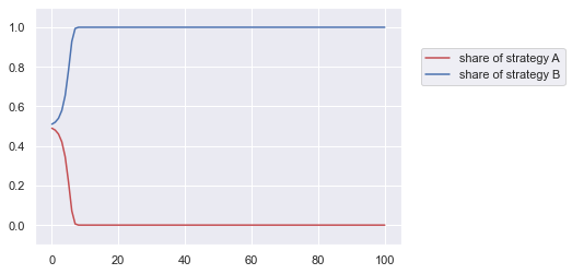
Replicator Dynamics
Consider a large population with \(N\) replicators. In each period, each replicator is randomly matched with another replicator for playing a two-players game.
Replicators are assigned strategies \(A\) or \(B\).
|
\(A\) |
\(B\) |
|---|---|---|
\(A\) |
\(a,a\) |
\(b,c\) |
\(B\) |
\(c,b\) |
\(d,d\) |
The proporition of the population playing strategy \(A\) is \(p_A\) and the proportion playing \(B\) is \(p_B\).
The state of the population is given by \((p_A, p_B)\) where \(p_A\ge 0, p_B\ge 0\) and \(p_A + p_B=1\).
Suppose that individuals are paired at random from a very large population to play the (bargaining) game. We assume that the probability of meeting a strategy can be taken as the proportion of the population that has that strategy. The population proportions evolve according to the replicator dynamics. The proportion of the population using a strategy in the next generation is the proportion playing that strategy in the current generation mutiplied by a fitness factor. This fitness factor is just the ratio of the average payoff to this strategy to the average payoff in the whole population.
import matplotlib.pyplot as plt
%matplotlib inline

# PD payoffs
#a = 3; b = 0; c = 4; d = 1

# SH payoffs
a = 4; b = 1; c = 3; d = 2

# Coord payoffs
a = 1; b = 0; c = 0; d = 1

pA = [0.49]
pB = [1 - pA[0]]

for t in range(100):

    fA = pA[t] * a + pB[t] * b
    fB = pA[t] * c + pB[t] * d
    f = pA[t] * fA + pB[t] * fB

    pA.append(pA[t] + (pA[t] * ((fA - f) / f)))
    pB.append(pB[t] + (pB[t] * ((fB - f) / f)))

plt.plot(pA, 'r', label ='share of strategy A')
plt.plot(pB, 'b', label ='share of strategy B')
plt.ylim(-0.1, 1.1)
plt.legend(loc='center', bbox_to_anchor=[1.25,0.75]);
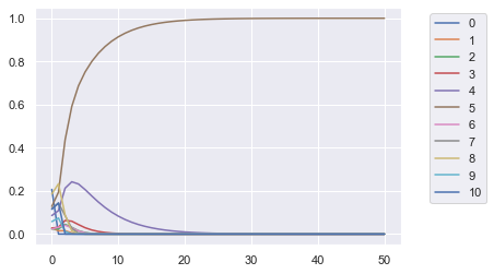
strats = [0, 1, 2, 3, 4, 5, 6, 7, 8, 9, 10]

init_probs = list(np.random.dirichlet((1,)* len(strats)))
#x0, x1, x2, x3, x4, x5, x6, x7, x8, x9, x10 = [0.0544685, 0.236312, 0.0560727, 0.0469244, 0.0562243, 0.0703294, 0.151136, 0.162231, 0.0098273, 0.111366, 0.0451093]
#x0, x1, x2, x3, x4, x5, x6, x7, x8, x9, x10 =  [0.410376, 0.107375, 0.0253916, 0.116684, 0.0813494, 0.00573677, 0.0277155, 0.0112791, 0.0163166, 0.191699, 0.00607705]
strat_probs = { strats[i]:[init_probs[i]] for i in range(len(strats)) }

print("Initial Probabilities", strat_probs)

def payout(s,other_s):

    return s if (s+other_s) <= 10 else 0


for t in range(50):

    fs = {s: sum(strat_probs[other_strat][t] * payout(s, other_strat)
                 for other_strat in strats)
          for s in strats}
    f = sum([strat_probs[s][t] * fs[s] for s in strats])

    for s in strats:
        strat_probs[s].append(strat_probs[s][t] + ((strat_probs[s][t] * (fs[s] - f)) / f))

threshold = 0.001

winning_strats = [s for s in strats if  strat_probs[s][-1] > threshold]
print(winning_strats)
for s in strats:
    plt.plot(strat_probs[s],   label = str(s))
plt.legend(loc='best', bbox_to_anchor=[1.25,1])

plt.show()
Initial Probabilities {0: [0.20707168045854377], 1: [0.028202979224481617], 2: [0.023794594376021147], 3: [0.027261546138785613], 4: [0.08574622794884816], 5: [0.12806079105412707], 6: [0.0233575830922005], 7: [0.11814882863611853], 8: [0.1856121078962921], 9: [0.05784506992092553], 10: [0.11489859125365585]}
[5]
import tqdm.notebook as tqdm

def payout(s,other_s):

    return s if (s+other_s) <= 10 else 0

def run_sim(strats):

    init_probs = list(np.random.dirichlet((1,)* len(strats)))

    strat_probs = { strats[i]:[init_probs[i]] for i in range(len(strats)) }

    for t in range(1000):

        fs = {s: sum(strat_probs[other_strat][t] * payout(s, other_strat)
                     for other_strat in strats)
              for s in strats}
        f = sum([strat_probs[s][t] * fs[s] for s in strats])

        for s in strats:
            strat_probs[s].append(strat_probs[s][t] + ((strat_probs[s][t] * (fs[s] - f)) / f))

    threshold = 0.001
    return sorted([s for s in strats if  strat_probs[s][-1] > threshold])

strats = [0, 1, 2, 3, 4, 5, 6, 7, 8, 9, 10]

num_converge = {
    (0,10): 0,
    (1, 9): 0,
    (2, 8): 0,
    (3, 7): 0,
    (4, 6): 0,
    (5,): 0
}

num_trials = 1000
for t in tqdm.tqdm(range(num_trials)):
    winning_strats = run_sim(strats)
    num_converge[tuple(winning_strats)] += 1
fig = plt.figure()
ax = fig.add_axes([0,0,1,1])

langs = ['(0,10)', '(1,9)', '(2,8)', '(3,7)', '(4,6)', '(5,5)']
students = [num_converge[(0,10)],
            num_converge[(1,9)],
            num_converge[(2,8)],
            num_converge[(3,7)],
            num_converge[(4,6)],
            num_converge[(5,)]]
ax.bar(langs,students)
plt.show()
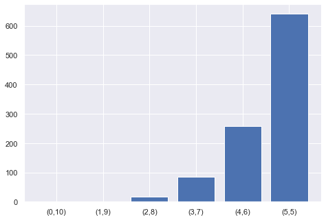
Suppose that every once and a while a member of the population just picks a strategy at random and tries it out—perhaps as an experiment, perhaps just as a mistake.
Suppose we are at a polymorphic equilibrium—for instance, the \((4,6)\) equilibrium. If there is some fixed probability of an experiment (or mistake), and if experiments are independent, and if we wait long enough, there will be enough experiments of the right kind to kick the population out of the basin of attraction of the \((4,6)\) polymorphism and into the basin of attraction of fair division and the evolutionary dynamics will carry fair division to fixation.
Peyton Young showed that, if we take the limit as the probability of someone experimenting gets smaller and smaller, the ratio of time spent in fair division approaches one.
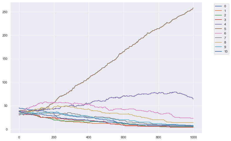
However, it is important to realise that the replicator dynamics assumes any pairwise interaction between individuals is equally likely. In reality, quite often interactions between individuals are correlated to some extent. Correlated interaction can occur as a result of spatial location (as shown above for the case of the spatial prisoner’s dilemma), the structuring effect of social relations, or ingroup/outgroup membership effects, to list a few causes.
from mesa import Model, Agent
from mesa.time import RandomActivation
from mesa.space import SingleGrid, NetworkGrid
from mesa.datacollection import DataCollector
import random
import nashpy as nash
import matplotlib.pyplot as plt
from IPython.display import clear_output
from ipywidgets import widgets, interact, interact_manual
import seaborn as sns
import numpy as np
import pandas
def payout(s,other_s):

    return s if (s+other_s) <= 10 else 0

class DivideDollarPlayer(Agent):
    '''
    A player for the divide th dollar game
    '''
    def __init__(self, unique_id, pos, model, strat):

        super().__init__(unique_id, model)
        self.pos = pos
        self.strat = strat # fixed strategy to play in the game

    def average_payout(self):
        '''find the average payout when playing the game against all neighbors'''
        neighbors = self.model.grid.neighbor_iter(self.pos)
        return np.average([payout(self.strat, n.strat) for n in neighbors])

    def total_payout(self):
        '''find the total payout when playing the game against all neighbors'''
        neighbors = self.model.grid.neighbor_iter(self.pos)
        return np.sum([payout(self.strat, n.strat) for n in neighbors])

    def step(self):
        pass

class DivideDollarLatticeModel(Model):
    '''
    Play a fixed game on a lattice.
    '''
    def __init__(self, height, width,  strats, num_changes_per_step, mutation, update_type, use_grid):

        self.height = height
        self.width = width
        self.strats = strats
        self.update_type = update_type
        self.num_changes_per_step = num_changes_per_step
        self.mutation = mutation

        self.use_grid = use_grid

        self.schedule = RandomActivation(self)
        self.grid = SingleGrid(height, width, torus=True)

        self.datacollector = DataCollector({
             "0": lambda m: np.sum([1 for a in m.schedule.agents if a.strat == 0]),
             "1": lambda m: np.sum([1 for a in m.schedule.agents if a.strat == 1]),
             "2": lambda m: np.sum([1 for a in m.schedule.agents if a.strat == 2]),
             "3": lambda m: np.sum([1 for a in m.schedule.agents if a.strat == 3]),
             "4": lambda m: np.sum([1 for a in m.schedule.agents if a.strat == 4]),
             "5": lambda m: np.sum([1 for a in m.schedule.agents if a.strat == 5]),
             "6": lambda m: np.sum([1 for a in m.schedule.agents if a.strat == 6]),
             "7": lambda m: np.sum([1 for a in m.schedule.agents if a.strat == 7]),
             "8": lambda m: np.sum([1 for a in m.schedule.agents if a.strat == 8]),
             "9": lambda m: np.sum([1 for a in m.schedule.agents if a.strat == 9]),
             "10": lambda m: np.sum([1 for a in m.schedule.agents if a.strat == 10]),
         } )
        self.running = True

        # Set up agents
        agent_id = 0
        for cell in self.grid.coord_iter():
            _,x,y = cell
            strat = random.choice(strats)
            agent = DivideDollarPlayer(agent_id, (x, y), self, strat)
            self.grid.position_agent(agent, x=x, y=y)
            self.schedule.add(agent)
            agent_id += 1


    def step(self):
        for i in range(self.num_changes_per_step):

            # choose a random agent
            focal_agent = np.random.choice(self.schedule.agents)


            # find all the neighbors of the agent

            if use_grid:
                neighbors = self.grid.get_neighbors(focal_agent.pos, moore=True)
            else:
                neighbors = random.sample(self.schedule.agents,8)

            if self.update_type == 'imitator':
                # imitate most successful neighbor
                total_payouts  = {a: a.total_payout() for a in neighbors}

                max_payout = max(total_payouts.values())

                strat_to_imitate = random.choice([a.strat for a in total_payouts.keys() if total_payouts[a] == max_payout])

            if self.update_type == 'prob_imitator':

                # get the average payouts for each neighbor
                average_payouts = [a.average_payout() for a in neighbors]
                total_average_payouts = np.sum(average_payouts)

                # probabilities for each neighbor
                neighbor_probs = [n.average_payout() / total_average_payouts for n in neighbors]

                # probabilistically imitate most successful neighbor
                strat_to_imitate = np.random.choice(neighbors, 1, p=neighbor_probs)[0].strat


            # mutations

            if random.random() < self.mutation:
                focal_agent.strat = random.choice([s for s in strats if s != strat_to_imitate])
            else:
                focal_agent.strat = strat_to_imitate

            self.datacollector.collect(self)

            self.schedule.steps += 1

        # stop running if all agents have the same strategy
        if len(list(set([a.strat for a in self.schedule.agents]))) == 1:
            self.running=False
strats = [0,1,2,3,4,5,6,7,8,9,10]

height, width = 20, 20
num_changes_per_step = 1
mutation = 0.0
update_type = 'imitator'
use_grid = True

m=DivideDollarLatticeModel(height,width,  strats, 1,  0.0, update_type, use_grid)

running = True
while running and m.schedule.steps < 1000:
    m.step()
    if len(list(set([a.strat for a in m.schedule.agents]))) == 1:
        running=False
df = m.datacollector.get_model_vars_dataframe()
df
| 0 | 1 | 2 | 3 | 4 | 5 | 6 | 7 | 8 | 9 | 10 | |
|---|---|---|---|---|---|---|---|---|---|---|---|
| 0 | 45 | 38 | 39 | 34 | 38 | 39 | 32 | 31 | 33 | 34 | 37 |
| 1 | 45 | 38 | 39 | 34 | 38 | 39 | 32 | 30 | 33 | 34 | 38 |
| 2 | 45 | 38 | 39 | 34 | 38 | 39 | 32 | 30 | 34 | 34 | 37 |
| 3 | 45 | 38 | 39 | 34 | 38 | 39 | 32 | 30 | 34 | 34 | 37 |
| 4 | 44 | 38 | 39 | 34 | 38 | 39 | 32 | 30 | 35 | 34 | 37 |
| ... | ... | ... | ... | ... | ... | ... | ... | ... | ... | ... | ... |
| 995 | 6 | 4 | 5 | 4 | 66 | 256 | 23 | 7 | 14 | 8 | 7 |
| 996 | 6 | 4 | 5 | 4 | 66 | 256 | 23 | 7 | 14 | 8 | 7 |
| 997 | 6 | 4 | 5 | 4 | 65 | 257 | 23 | 7 | 14 | 8 | 7 |
| 998 | 6 | 4 | 5 | 4 | 64 | 258 | 23 | 7 | 14 | 8 | 7 |
| 999 | 6 | 4 | 5 | 4 | 64 | 258 | 23 | 7 | 14 | 8 | 7 |
1000 rows × 11 columns
sns.set(rc={'figure.figsize':(11.7,8.27)})
for s in strats:
    plt.plot(list(df[str(s)]), lw=2, label = str(s))

plt.legend(loc='best', bbox_to_anchor=[1.15,1]);
Further Reading
J. McKenzie Alexander (2000). Evolutionary Explanations of Distributive Justice, Philosophy of Science, vol. 67, pp. 490 - 516
J. McKenzie Alexander (2009). Social Deliberation: Nash, Bayes, and the Partial Vindication of Gabriele Tarde, Episteme, 6(2), pp. 164 - 184.